
Nuclear Shell model code BIGSTICK
Last update: April 22, 2024
Intro
BIGSTICK (Calvin, et al) is large scale nuclear shell model code written in FORTRAN. It can calculate energy spectrum, one-body density matrix, and expectation value of operator. This is particularly important for the study of nucleus scattering. This writeup illustrate the usage of BIGSTICK and the relationship between it and nucleus scattering. This writeup is organized as follows: nuclear physics, installation, preparation of the inputs, and interpretation of the outputs. We will not discuss about any algorithm as it’s rather clearly described in BIGSTICK manual.
Nuclear physics
Nuclear quantum number
A nucleus is made of protons and neutrons. For example $^{12}{\rm C}$ has 6 protons and 6 neutrons, $^{133}{\rm Cs}$ has 55 protons and 78 protons. That is, nucleus is a many-fermion system. There is no analytical solution in any literature (except simple enough nucleus like hydrogen and helium). Thus we have to have a numerical calculator. One of the famous model is nuclear shell model. Just like Bohr model (hydrogen atom model), it formulates the nucleons into a serial of shells. Each shell has 4 quantum number.
- nodal (radial) quantum number $n$
- principal quantum number $N$
- orbital angular quantum number $l$
- total angular quantum number $j$
Note that in some notation $n$ starts from 1. In particular $l$ has special notation:
| $l$ notation | s | p | d | f | g |
|---|---|---|---|---|---|
| $l$ value | 0 | 1 | 2 | 3 | 4 |
and so on
Nuclear shell
To label a shell, we use the following notation
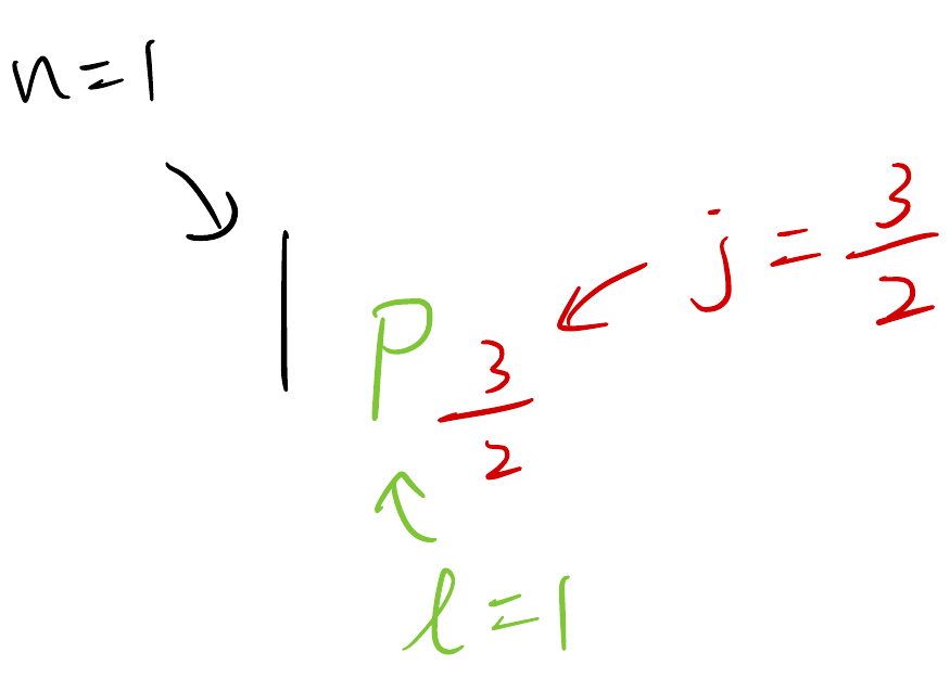
A shell spectrum looks like this
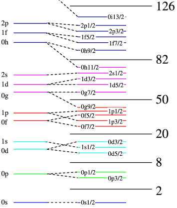
The bottom has the lowest energy. Since there exists relatively large gap between the shells with the number box, we often group them together and call it shell model space or shell model orbit
| model space | components |
|---|---|
| s | $0s_{1/2}$ |
| p | $0p_{1/2}$, $0p_{3/2}$ |
| sd | $1s_{1/2}$, $0d_{5/2}$, $0d_{3/2}$ |
| pf | $1p_{1/2}$, $1p_{3/2}$, $0f_{7/2}$, $0f_{5/2}$ |
If the nucleons are full in these spaces, then one extra nucleon needs high energy to fill. Thus in this case the nucleus is stable. 2, 8, 20, 28, 50 are the (nuclear) magic number
In most of the experiments, nucleus is initially in ground state $J_i$. After the scattering, the nucleus may be excited to a certain excited state $J_f$. In which we are interested in the excitation energy $\Delta E$ and the probability of the transition (density matrix to be more precise). See the next section for how to use BIGSTICK to compute excitation energy and density matrix.
Nuclear operator and transition
Occasionally we are looking for the expectation value of an operator $\hat{O}$, say spin $\hat{\sigma}$ or Gamow-Teller $\hat{\sigma} \hat{\tau}$. That is, we want to calculate
\[\langle J_f | \hat{O} | J_i \rangle\]Such calculation is also supported by BIGSTICK, see next section for details.
Install BIGSTICK
$ git clone https://www.github.com/cwjsdsu/BigstickPublick/
$ cd BigstickPublick/src
$ nano Makefile # or other editor like vim or sublime text

# run only one of the following
$ make serial  # build serial BIGSTICK in default compiler
$ make gfortran # use gfortran to compile BIGSTICK (serial)
$ make openmp-mpi # build parallel BIGSTICK in OpenMP + MPI

# Or use make help to see the options
$ make help
If sucessfully installed, there will be an executable ending in .x, such as bigstick.x, bigstick-mpi.x, depending on the compilation method.
$ ls -l | grep bigstick
-rw-r--r-- 1 wei-chih wei-chih  33K Nov  2  2021 bigstick_main.f90
-rw-rw-r-- 1 wei-chih wei-chih  71K Jun  7  2022 bigstick_main.o
-rw-r--r-- 1 wei-chih wei-chih 624K Nov  2  2021 BIGSTICK_Manual.pdf
-rwxrwxr-x 1 wei-chih wei-chih 2.0M Jun  7  2022 bigstick.x
Input files
The input files are specific to the nucleus. They also determines how long and how heavy the calculation will be. The lines starting with $!$ are treated as comments and will be ignored in calculation.
Particle space (.sps)
Particle space file define the Hilbert space for the nucleus, ending in .sps. Each row represents one orbit and has 4 numbers, $n$, $l$, $j$ and weight, separated in space. Weights are any non-negative number used to do a more sophisticated job.
! 0p.sps
iso    ! isosymmetry
2      ! there are 2 orbits
       0.0  1.0  0.5  1  ! n=0, l=1, j=0.5, weight=1
       0.0  1.0  1.5  1  ! n=0, l=1, j=1.5, weight=1
Below is an example of a different weighted orbits. Protons are on the top, neutron are at the bottom.
! Ar40 orbits
iso
7
       0.0  2.0  1.5  1  ! protons
       0.0  2.0  2.5  1
       1.0  0.0  0.5  1
       0.0  3.0  3.5  0
       1.0  1.0  1.5  0
       0.0  3.0  2.5  0
       1.0  1.0  0.5  0
       0.0  2.0  1.5  0  ! neutrons
       0.0  2.0  2.5  0
       1.0  0.0  0.5  0
       0.0  3.0  3.5  1
       1.0  1.0  1.5  1
       0.0  3.0  2.5  1
       1.0  1.0  0.5  1
Alternatively one can have a different weight distribution.
iso
7
       0.0  2.0  2.5  1
       1.0  0.0  0.5  1
       0.0  2.0  1.5  2
       0.0  3.0  3.5  3
       1.0  1.0  1.5  3
       0.0  3.0  2.5  4
       1.0  1.0  0.5  4
       0.0  2.0  2.5  0
       1.0  0.0  0.5  0
       0.0  2.0  1.5  0
       0.0  3.0  3.5  1
       1.0  1.0  1.5  1
       0.0  3.0  2.5  1
       1.0  1.0  0.5  1
For heavy nucleus like Sn, Cs, Xe, etc, I often use the sps below, which includes the pink region in the shell spectrum.
! jj5pn.sp used to be sn100pn.sps
pn
100 50    ! A,Z of core
10        ! number of orbits
2 5 5     ! number of species, orbits per species
1 1 4 7   ! index, n, l, 2j
2 2 2 5
3 2 2 3
4 3 0 1
5 1 5 11
6 1 4 7
7 2 2 5
8 2 2 3
9 3 0 1
10 1 5 11
Interaction (*.int)
The interaction file (*.int) defines the Hamiltonian of the potential. It does not look as simple as particle space orbit. Often time we simply take open source interaction files from the existing literature, or use other numerical software to generate. For example, usdb.int is the interaction for the orbits $0d_{3/2}$, $0d_{5/2}$, $1s_{1/2}$. First line contains the number of nonzero elements and the energy of the described orbits. The rest of the file are two body matrix element $V_{JT}(ab,cd)= \langle ab; JT | V | cd; JT \rangle$, V is the nuclear potential $a,b,c,d$ are the label of nucleus, J/T is the spin/isospin
! 1=d3/2 2=d5/2 3=s1/2 (must match with .sps)
! total 63 orbits, else are the orbit energies
63 2.1117 -3.9257 -3.2079

! two body matrix elements
! a  b  c  d    J  T   V
  2  2  2  2    1  0  -1.3796
  2  2  2  1    1  0   3.4987
  2  2  1  1    1  0   1.6647
  2  2  1  3    1  0   0.0272
  2  2  3  3    1  0  -0.5344
  ...
The orbit order must match with the particle space file.
Strength operator (*.opme)
Suppose we want to calculate $\langle J_f | \hat{O} | J_i \rangle$. We will need a file for matrix elements just like the interaction file. For example, below is the spin operator elements for psd orbit.
! psd_spin.opme
iso
 5   ! number of orbits
  1    0    1    0.5  ! orbit label, n, l, j
  2    0    1    1.5
  3    0    2    1.5
  4    0    2    2.5
  5    1    0    0.5
1     0   ! J, T
    1    1  -1.15470046955374  ! <orbit 1| spin |orbit 1> = -1.15
    1    2  3.26598612904295   ! <orbit 1| spin |orbit 2> = 3.26
    2    1  -3.26598612904295
    2    2  3.65148403628416
    3    3  -2.19089042177050
    3    4  4.38178092104527
    4    3  -4.38178092104527
    4    4  4.09878016621536
    5    5  3.46410161513776
The orbit label always starts from 1.
Input script (*.in)
There are two ways to use BIGSTICK.
Interactive mode:
Enter
$ YOURS/BigstickPublick/src/bigstick.xin terminal, then this shows up
  BIGSTICK: a CI shell-model code, version 7.10.4Nov  2021

  Please cite: C. W. Johnson, W. E. Ormand, and P. G. Krastev
  Comp. Phys. Comm. 184, 2761-2774 (2013);
  and C. W. Johnson, W. E. Ormand, K. S. McElvain, H.-Z. Shan
   arXiv:1801.08432 and report UCRL LLNL-SM-739926

  This code distributed under the MIT Open Source License

 Running on NERSC_HOST: none, scratch_dir (*.wfn,...): .
 Number of MPI processors =           1 , NUM_THREADS =            1

  * * * * * * * * * * * * * * * * * * * * * * * * * * * * * * * * * * * * * *
  *                                                                         *
  *               OPTIONS (choose one)                                      *
  * (i) Input automatically read from "autoinput.bigstick" file             *
  *  (note: autoinput.bigstick file created with each nonauto run)          *
  * (n) Compute spectrum (default); (ns) to suppress eigenvector write up   *
  * (j) Carry out jumpstart run to set MPI timing (MPI only)                *
  * (d) Densities: Compute spectrum + all one-body densities                *
  * (2) Two-body density from previous wfn (default p-n format)             *
  * (x) eXpectation value of a scalar Hamiltonian (from previous wfn)       *
  * (o) Apply a one-body (transition) operator to previous wfn and write out*
  * (s) Strength function (using starting pivot )                           *
  * (g) Apply the resolvant 1/(E-H) to a previous wfn and write out         *
  * (m) print information for Modeling parallel distribution                *
  * (l) print license and copyright information                             *
  * (?) Print out all options                                               *
  *                                                                         *
  * * * * * * * * * * * * * * * * * * * * * * * * * * * * * * * * * * * * * *

  Enter choice
Then simply follow the instructions and enter what it asks.
- Script mode Once you are familiar with inputs, you can put the inputs together in one single file
create_wfn.in
! create_wfn.in
d             ! create densities
f19           ! output name
sd            ! orbit information (sd.sps)
1 2           ! # of valence protons, neutrons (compare to O16)
1             ! 2 * jz(spin of nucleus)
usdb          ! interaction file name (usdb.int)
1 18. 19. 0.3 ! scaling, 1 for single particle energy, 18 for core mass number+2, 19 for target mass (p.44 in document)
end           ! end of reading in Hamiltonian files
ex            ! 'exact' or full diagonalization by Householder rather than Lanczos
20            ! 1 states kept (max # iterations for lanczos)
Notice that the orbit and interaction file do not end with .sps or .int in the input script. To compute the operator expectation value, one needs two scripts, create_strength.in and create_operator.in
! create_operator.in
o                ! Apply a one-body (transition) operator
f19              ! previous run wfn
f19_o            ! output name
sd_f0            ! .opme file
! create_strength.in
s                ! Compute strength function distribution using previous wfn
f19_o            ! previous run wfn
f19_s            ! output name
usdb             ! interaction file
1 18. 19. 0.3    ! scale
end
200 200          ! # of state, lanczos iterations
1                ! pivot vector
In create_strength.in, number of state should be equal to Lanczos iterations, and pivot vector is the $J_i$ in $\langle J_f | \hat{O} | J_i \rangle$
Once these input scripts are ready, we can type the following to run
$ your_bigstick.x < create_wfn.in  # stop here if you just need the densities
$ your_bigstick.x < create_operator.in
$ your_bigstick.x < create_strength.in
Note that it’s necessary to follow this order.
I wrote a python script to generate BIGSTICK input script, see this post
Output files
*.wfn
BIGSTICK internal wavefunction binary, not human readable. It can be input to BIGSTICK to do further calculations.
*.res
f19.res energy, spin, isospin spectrum
  BIGSTICK Version 7.10.4Nov  2021
  single-particle file = sd
           1           2
           1 +
  State      E        Ex         J      T
    1    -23.86096   0.00000     0.500   0.500
    2    -23.78367   0.07729     2.500   0.500
    3    -22.09059   1.77037     1.500   0.500
    4    -21.26237   2.59859     4.500   0.500
    5    -19.25724   4.60371     6.500   0.500
    6    -18.99335   4.86761     3.500   0.500
...
State is the state number, 1 is ground state, 2 is first excited state, and so on. E is absolute state energy, Ex is excitation energy, both in MeV J is spin, T is isospin.
f19_s.res expectation value of the operator given in .opme file
  BIGSTICK Version 7.10.4Nov  2021
           1           2
           1 +
  0.13035753317112964       = total strength
         127  iterations

  Energy   Strength
  ______   ________
  -23.860957    0.041220
  -23.783670    0.000000
  -22.090586    0.000014
  -21.262371    0.000000
  -19.257241    0.000000
  -18.993350    0.000000
  -18.891616    0.000000
...
Energy is absolute state energy (same as f19.res), strength is the sqaured of expectation value $| \langle J_f | \hat{O} | J_i \rangle |^2$ in whatever unit defined in .opme file.
*.dres
f19.dres reduced one-body densities matrix $\rho^{fi}_K(a^\dagger b) = [K]^{-1} \langle J_f || (a^\dagger b)_K || J_i \rangle$
...
 Initial state #    1 E =  -23.86096 2xJ, 2xT =    1   1
 Final state   #    1 E =  -23.86096 2xJ, 2xT =    1   1
 Jt =   0, Tt = 0        1
    1    1   0.19126   0.02824
    2    2   0.89604   0.34888
    3    3   1.17753   0.35578
 Jt =   1, Tt = 0        1
    1    1  -0.05634   0.01600
    1    2   0.13395  -0.10506
    1    3  -0.01476  -0.01563
    2    1  -0.13395   0.10506
    2    2   0.12703  -0.24666
    3    1   0.01476   0.01563
    3    3   0.42662  -0.39164
...
For example,
1 3 -0.01476 -0.01563
1 is the label of the first orbit, 3 is the 3rd, defined in .sps file.
The one-body matrix elements are
\[-0.01476 = \langle \Phi_2 || [a_1^\dagger a_3]_{J=1,T=0} || \Phi_1 \rangle \\ -0.01563 = \langle \Phi_2 || [a_1^\dagger a_3]_{J=1,T=1} || \Phi_1 \rangle\]Hands-on example
Download the folder and run
$ cd F19/
$ YOURS/BigstickPublick/src/bigstick.x < create_wfn.in
$ YOURS/BigstickPublick/src/bigstick.x < create_operator.in
$ YOURS/BigstickPublick/src/bigstick.x < create_strength.in
Then
f19.res(energy state spectrum)f19.dres(density matrix)f19_s.res(strength for Gamow-Teller)
will be generated.
Other nuclei examples are included in folder
Conclusion and afterword
Now you are ready to compute almost every kind of nucleus. All you need is to find the suitable interaction file (.int).
Depending on the nucleus, it could be extremely heavy to calculate, especially for heavy nuclei. The following is the computational cost for what I’ve calculated,
| nucleus | Time | RAM | CPU |
|---|---|---|---|
| Ar40 | a few minutes | a few GB | 1 |
| Cs133 | 4hr | 3TB | 384 |
| I127 | 5.5hr | 13TB | 1680 |
To get more practical and meaningful outcomes after BIGSTICK, there is still some work to do. See 7operator for how to turn BIGSTICK output to response functions and cross sections.
Obviously BIGSTICK is capable of doing more than this post. Refer to the manual for details.